Monte Carlo Simulation in Excel: A Complete Guide

Monte Carlo methods, originally named after the Monte Carlo Casino in Monaco, are widely used in fields such as finance, engineering, supply chain, and science to model phenomena with significant uncertainty in their inputs.

But what is Monte Carlo simulation? How does it work? And how can I implement the simulation and analyze the results?

This tutorial will introduce you to the Monte Carlo simulation and the relevant statistical concepts behind the technique. We will also implement the Monte Carlo simulation in Excel, familiarizing you with relevant Excel built-in functions.

Finally, the tutorial will leave you with best practices, advanced techniques, and further resources, making this tutorial your one-stop guide to learning everything about Monte Carlo simulation in Microsoft Excel.

What is Monte Carlo Simulation?

Monte Carlo Simulation is a mathematical technique used to model the probability of different outcomes in a process that cannot easily be predicted due to the intervention of random variables.

It’s a powerful tool for understanding the impact of risk and uncertainty in various fields. The method relies on repeated random sampling to simulate the behavior of complex systems and processes.

The problem is first modelled by a probability distribution for each variable that has inherent uncertainty. Large numbers of random samples are then drawn from these probability distributions, and these samples are used to compute the outcomes. This process is repeated many times to create a distribution of possible outcomes, which can be analyzed statistically to provide predictions about how a system will behave.

So, in simple terms. Monte Carlo simulation is a technique that predicts how complex systems will behave by simulating their outcomes many times using random values. It uses several steps:

• Model uncertainty: Define how each variable can vary using probability distributions.
• Random sampling: Randomly select values for these variables based on their distributions.
• Simulate outcomes: Use these values to simulate the system's behavior.
• Analyze results: Repeat the process many times to get a range of possible outcomes, then analyze these to predict the most likely scenarios.

Next, we’ll build up our basic understanding of Monte Carlo simulation by delving into some relevant statistical concepts.

Understanding Random Variables and Probability Distributions

Random variables and their associated probability distributions are fundamental to Monte Carlo simulation as they provide the mathematical framework for modeling and simulating the randomness and variability inherent in complex systems.

Random variables

A random variable is a variable whose values are outcomes of a random phenomenon.

Random variables are classified into two types:

• Discrete random variables: These variables take on a countable number of distinct values. In simulations, discrete variables might model scenarios like the number of defective items in a batch, customer arrivals per hour, or other countable events.
• Continuous random variables: These variables can take on any values in a continuous range. Continuous variables are used for simulations dealing with physical measurements or time durations.

Random variables are used in simulations because they contain the uncertainty that Monte Carlo techniques are designed to explore and quantify.

Probability distributions

Probability distributions describe how the probabilities are distributed over the values of a random variable.

Probability distributions are used in Monte Carlo simulation to define how different inputs or scenarios are expected to behave, which is essential for accurate modeling and decision-making.

Normal distribution is the most commonly used distribution in statistics and simulations because many natural and human-made phenomena tend to follow this distribution due to the Central Limit Theorem.

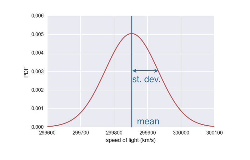
Normal distribution (Source)

Normal distribution is used for modeling variables that are influenced by many small, independent effects, such as measurement errors or stock market returns.

Some other probability distributions are uniform distributions which are used when any outcome in a specified range is equally likely — a common assumption in simulations when no prior data is available, and binomial distributions, which are used when modeling scenarios with two possible outcomes (success/failure) across a series of experiments, such as pass/fail testing or quality control checks.

Now that we have understood the concepts and theory behind Monte Carlo simulations, let’s move into the implementation side of things.

Why Use Excel for Monte Carlo Simulation?

Once you have chosen to implement a Monte Carlo simulation, you have multiple tools, such as Excel, Python, R, SAS, and MATLAB, to help you with the simulations.

The most important factor to consider, especially when implementing Monte Carlo simulation for the first time, is your overall familiarity with the tool. Excel is one of the most widely used tools in the business world, which means many people are already familiar with its basic operations. This reduces training time and eliminates the need to learn new software from scratch.

Excel also provides easy-to-use tools for creating charts and graphs, which can be useful for visualizing the results of simulations. In addition, several powerful add-ins are available for Excel, enhancing its capability to perform complex Monte Carlo simulations.

However, it’s also worth noting that for more advanced simulations, especially those requiring handling large datasets or running a very high number of simulations, more specialized tools other than Excel might be more appropriate.

Overview of Relevant Excel Functions

Next, we will explore two essential Excel functions: RAND and NORM.INV, covering their syntax, parameters, and typical use cases. These functions help generate random numbers and define probability distributions, which are fundamental aspects of any simulation.

The syntax and parameters for the RAND function

RAND generates a random number greater than or equal to 0 and less than 1. The numbers are uniformly distributed, meaning any number within the specified range is equally likely to occur.

The syntax for RAND is as follows:

RAND()

The RAND function does not require any arguments. It's used simply as RAND().

In the context of the Monte Carlo Simulation, RAND() can be used to simulate the occurrence of random events or to vary the inputs into your model.

The syntax and parameters for the NORM.INV function

While RAND generates uniform random numbers, NORM.INV is used to generate random numbers from a normal distribution, which is a common requirement in a Monte Carlo Simulation. This function returns the inverse of the normal cumulative distribution for a specified mean and standard deviation.

The syntax for NORM.INV function is as follows:

NORM.INV(probability, mean, standard_deviation)

The parameters are:

• probability: A probability corresponding to the normal distribution, which must be a value between 0 and 1. This is typically generated by the RAND() function.
• mean: The arithmetic mean of the normal distribution.
• standard_deviation: The standard deviation of the normal distribution, a measure of how spread out the numbers are around the mean.

The NORM.INV is used to transform uniformly distributed random numbers from the RAND function into numbers that follow a specified normal distribution. This becomes useful for modeling variables that are expected to exhibit natural variability following a normal curve.

Now that we have all the building blocks, functions, and concepts behind a Monte Carlo simulation, let’s implement one in Microsoft Excel.

Implementing Monte Carlo Simulation in Microsoft Excel: An Example

Consider a scenario where you’re a data analyst working in a dynamic consumer electronics company and have been tasked with assessing the financial viability of launching a new wearable fitness tracker.

The market for such devices is competitive and consumer demand can be highly variable, influenced by seasonal trends, marketing effectiveness, and competitor actions. Additionally, the costs associated with manufacturing these devices are subject to fluctuations due to changes in material costs and supply chain uncertainties.

You have decided to use Monte Carlo simulation in Excel to address these challenges. You believe this approach will help you estimate potential profitability under different scenarios, enabling the company to make well-informed decisions about pricing strategies, production volumes, and marketing investments.

You have also analyzed past data from similar product launches and market studies within the consumer electronics industry. From this analysis, you have concluded certain metrics that will inform your simulation:

• An average demand of 10,000 units for new devices within the first year of launch, with a standard deviation of 2,000 units, reflecting the uncertainty in consumer uptake.
• Unit sale price typically ranges between $50 and $70, depending on competitive pricing and market saturation.
• The unit cost, influenced by volatile material prices and manufacturing efficiency, averages $30 per unit with a standard deviation of $5.

This historical data forms the underlying assumptions of your simulation parameters, helping to create the simulation to reflect current market conditions more accurately.

The steps you could follow to implement the Monte Carlo simulation for this particular example are as below:

Step 1: Set up your Excel sheet

First, prepare your Excel worksheet to include columns for each variable and a column for the calculated profit.

Here’s how it would look initially:

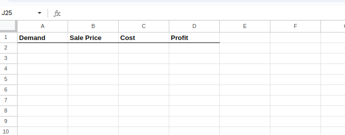
Setting up the Excel sheet.

Step 2: Input formulas for variables

In each row, you’ll input formulas to generate random values for demand, sale price, and cost based on the distributions you’ve identified:

• Demand: Normal distribution (mean = 10,000 units, standard deviation = 2,000 units)
• Sale Price: Uniform distribution ($50 to $70)
• Cost: Normal distribution (mean = $30, standard deviation = $5)

To input these formulas one by one, select cell A2 and type the following:

=NORM.INV(RAND(), 10000, 2000)

The above equation creates a normal distribution with a given mean and standard deviation as below:

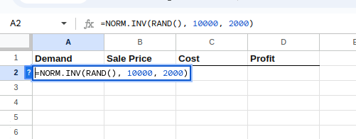
Creating the distribution for demand.

Next, select cell B2 and type in the following:

=50 + (70-50) * RAND()

The equation above creates a uniform distribution between $50 and $70 for the selling price as below:

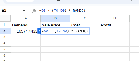
Creating the distribution for selling price.

Select cell C2, and type the following:

=NORM.INV(RAND(), 30, 5)

The equation above, similar to the demand equation, creates a normal distribution with a given mean and standard deviation as below:

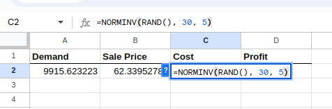
Creating the distribution for cost.

Step 3: Calculate the dependent variable

Now, calculate the profit, which is the dependent variable, for each simulation using the formula in column D:

=(B2 - C2) * A2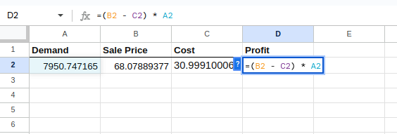

Calculating the profit.

Step 4: Fill down to simulate multiple scenarios

What we have so far done is to create a single simulation. Let us extend it to multiple, let’s say a thousand simulations.

Select cells A2 to D2 and drag the fill handle (a small square at the bottom-right of the selection) down to fill the formulas through as many rows as you want to simulate (e.g., 1000 rows for 1000 simulations).

It will look something like this:

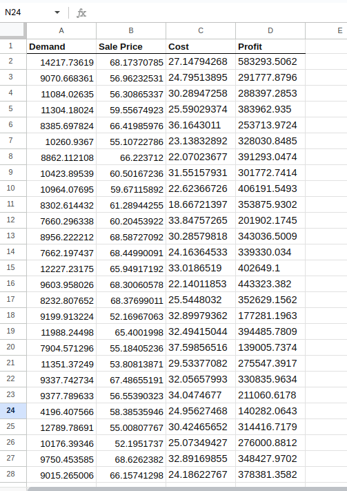
Creating the simulations.

Step 5: Analyze the results

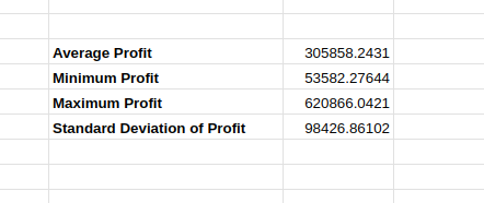
After running the simulations, you can analyze the results using statistical functions such as min, max, average, and standard deviations. Don’t hesitate to quickly refer to the Excel cheat sheet for a refresher on the built-in Excel functions we’ll use next.

To find the average profit expected each month, type the following in a cell, say G6:

=AVERAGE(D2:D1001)

To find the minimum profit expected each month, type the following in a cell, say G7:

=MIN(D2:D1001)

To find the maximum profit expected each month, type the following in a cell, say G8:

=MAX(D2:D1001)

To find the standard deviation of profit, type the following in a cell, say G9:

=STDEV.P(D2:D1001)

Once executed, the Excel sheet should look something like this:

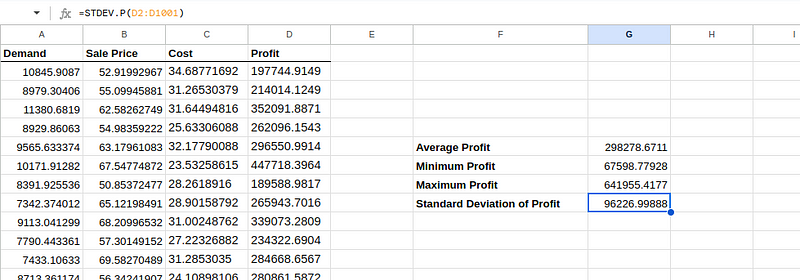
Analyzing the simulation results.

We can interpret the estimated results and the implications for the product launch as below:

• The average profit figure represents the expected profit from launching the new fitness tracker. It suggests that, on average, each simulation run predicts that we could expect to make around $298,278.67 in profit. This value is useful as a central estimate of profitability under the given assumptions.
• A minimum profit of $67,598.78 is the lowest profit observed across all our simulations. It indicates the worst-case scenario under your model’s assumptions, which is still profitable but significantly less so than the average. This could be due to particularly low demand or unfavorable cost conditions in that specific simulation.
• A maximum profit of $641,955.42 represents the best-case scenario, where demand and price were likely at their highest and costs at their lowest across all simulations. This shows the potential upside if conditions turn out to be highly favorable.

Given the wide range between the minimum and maximum profits and the substantial standard deviation, there’s considerable financial risk associated with launching the new product.

Decision-makers should consider whether the company is comfortable with this level of uncertainty and the potential for lower-than-average profits.

Further, though it’s optional, we encourage you to create visualizations such as Histograms to have a visual understanding of the results of the simulations.

Best Practices & Advanced Techniques to Improve the Simulations

When you re-run the same simulation as above, you can observe a slight difference in the calculations, as shown below:

Varying simulation results.

This is because the values of the original simulation can change between iterations, influencing the resulting estimations. Though the variation is small, when the estimated value changes, a concern about the accuracy and reliability of the simulation arises in the minds of the decision-makers.

Let us explore a few advanced techniques that we could use to improve the accuracy and reliability of the simulations.

Increasing the number of simulations

Running a larger number of simulations helps average out random fluctuations and provides a more stable and accurate estimate of the outcomes.

For the example above, we can increase the number of simulation runs (e.g., from 1,000 to 10,000 or more), especially when dealing with highly variable parameters.

Determining the “right” number of simulations depends on several factors.

The more complex the model (i.e., the more variables and the wider the range of their interactions), the more simulations are typically needed to capture all possible outcomes and ensure that the results are not due to chance.

If the inputs have high variability or are heavily skewed, more simulations will be necessary to accurately estimate the tails (extreme values) of the outcome distributions.

For more detailed analyses, particularly in finance or risk management, it is not uncommon to run 10,000 to 100,000 simulations. This range is typically used to ensure robust results across various scenarios and inputs. Of course, as we mentioned previously, for such large-scale analysis, Excel is not always the best choice of tool, rather R or Python.

Refining the input distributions

The accuracy of the simulations largely depends on how well the input probability distributions reflect the true uncertainty and behavior of the underlying variables. In our example above, we assumed a normal distribution for demand and cost and a uniform distribution for sales price.

Additionally, we could analyze more comprehensive historical data to parameterize the distributions better. We can better understand the behaviors of cost, sale, and demand on external factors based on domain expert input. We can also consider using distributions like log-normal, beta, or gamma or creating custom distributions based on empirical data.

Conducting a sensitivity analysis

This analysis is done to understand which input variables have the most significant impact on the output by systematically varying each input while holding others constant.

In our example above, we can hold two variables constant and change one’s distribution to understand the changes in the estimates. Then, repeat the same process to the remaining two variables one by one. Eventually, this technique helps in understanding which variable to focus efforts on to improve accuracy.

Employing the above techniques iteratively and analyzing the results can lead to more accurate and reliable results.

Conclusion

This tutorial introduced you to the Monte Carlo Simulation and the relevant statistical concepts. After introducing relevant Excel functions, the tutorial provided a step-by-step guide to implement the Monte Carlo Simulation in Excel using a real-world example.

Finally, you learned about some best practices and advanced techniques to ensure your results are more accurate and reliable.

If you’re particularly interested in implementing the above Monte Carlo Simulation using other tools such as Python or R, these two resources would be of use:

• Monte Carlo Simulations in R
• Monte Carlo Simulations in Python

Alternatively, if you’d like to stick to the familiar Microsoft Excel, and would like to master your skills using the widely adopted tool, you would want to check out the Excel Fundamentals track.